User Tools

Site Tools


processing:compute_gvectors

Compute G-vectors

G-vectors are the scattering vector associated with the diffraction. The are nodes of the reciprocal space or, in direct space, normal to the diffracting plane.

For a given reflection in the crystal, Ghkl is perpendicular to the diffracting plane (hkl) and its norm is 2π/dhkl. Pay attention, however, as some authors do not include the 2π factor in the calculation of G. In this case, the norm of Ghkl is 1/dhkl. For a detailed discussion: 2π or not?

The real space coordinates of Ghkl can be calculated from the experimental measurements, namely the x-ray wavelength λ, the diffraction angle 2θ, the azimuth angle η, and the rotation angle ω (see section on experiment geometry) and the detailed calculation in fable_geometry_version_1.0.8.pdf.

The x-ray wavelength λ is known, so is the rotation angle ω. There are issues, however, to evaluate the diffraction angle 2θ and the azimuth angle η. What is measured is the location of a diffraction spot on a detector. Calculating 2θ and η from the location of a diffraction spot on a detector requires calibration.

This step is typically performed with ImageD11.

O-Matrix

At this point, you should know the O-Matrix of your experiment. If not, go back to the section on understanding the concept of the O-Matrix.

Loading peaks

For calculating the G vectors, we use ImageD11. The software can be started by typing the following command in a terminal:

 ImageD11_gui.py

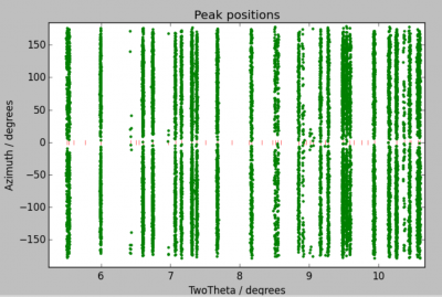
Peaks found during peak search can be loaded by clicking on Transformation –> Load filtered peaks and choosing the corresponding .flt file. You can display the peaks by calling the corresponding menu item in Transformation. You can either plot peaks in the 2D diffraction geometry (y/z plot), or after transforming detector peak positions into diffraction 2θ and the azimuth η angles (2θ/η plot).

If things look weird after you switch from (y/z) to 2θ/η plots of vice-versa, trying calling the Clear plot button at the bottom of the interface. Clear does only erase the plot, the data is still there.

ImageD11 Calibration

Preferably, this step should be performed with data collected on calibrant, for which you are sure of the unit cell parameters, which is free of strain, and with a controlled microstructures.

In diamond anvil cell beamlines, this step is often performed with a CeO2 or a LaB6 standard.

Go in to Transformation –> Edit parameters and enter all parameters you know. These include

  • the sample symmetry and unit cell parameters,
  • the O-Matrix,
  • the x-ray wavelength,
  • the sample to detector distance,
  • information on beam center.

Because of different conventions used by different softwares, the beam center might change from your calibration (in Fit2D, Dioptas, or anything you use). For instance, if have a 2048×2048 pixels image and found a beam center at 1000 and 900 during calibration, the correct value in ImageD11 should be one of 1000, 900, 1048, or 1148. Use the 2θ/η plot in order to see which one works.

Most of the peaks should appear to be on imaginary vertical lines. Zoom in and check, if these lines are actually vertical. If not, you might

  • have strain in your sample,
  • have a wrong beam center,
  • need to refine the detector tilts.
ImageD11 plotting peaks in the 2θ/η plot. After calibration, and if your sample is not strained, these should appear as straight lines. Predicted unit cell peaks positions are in red. ImageD11 crystallography is not complete. There are more predicted peaks that in the actual sample.

At this point, you should click on Transformation –> Add unit cell peaks. Red tick marks will appear which indicate the expected positions of the vertical lines. With this you can check whether your input parameters (cell parameters, detector distance, …) are correct.

If you sample is strained, there is nothing you can do beyond this step. Your calibration of ImageD11 should have been done beforehand.

If not, you a ready for a final refinement of the experimental parameters. You should start by refining the tilt_y and tilt_z, for accounting for the tilting of the detector. In the parameters window, check the marks next to both parameters, hit save, and click on Transformation –> Fit multiple times until the spots don't move anymore. You can also try to improve your beam center using the same procedure (although it should be good already).

At the end of the calibration, the imaginary lines should now be completely straight (if you don't have strain). If they are not, you have more work to do.

Save the experimental parameters with Transformation –> Save Parameters, with a .prm extension preferably. You will be able to use those for the rest of the processing of the current experiment.

You are ready for G-vectors calculations.

Computing G-vectors with ImageD11

Once ImageD11 has been calibrated,

  1. load your peaks (e.g. the .flt file from the peak search,
  2. make sure the ImageD11 parameters are ok or load them using Transformation –> Load Parameters ,
  3. Click Transformation –> Compute g-vectors(nothing will happen)
  4. Click Transformation –> Save g-vectors and save your list of g-vectors with a .gve extension.

ImageD11 will use the experimental wavelength, the rotation angle ω, and the positions of the peaks on the detector in order to compute the coordinates of each g-vector in the laboratory reference frame.

Note that, at this point, ImageD11 does not use any crystallography information. The calculations of g-vectors is a geometric operation. It is ok if the sample properties (e.g. cell lattice and parameters) in the parameter file does not match you sample. G-vectors will be correct.

While indexing grains, however, the header with crystallographic information (i.e. cell parameters and information about fitting reflections) will be used.

Optional step: evaluating g-vectors

In ImageD11, you click on Indexing > load g-vectors and load your gve file. You can then select Indexing > Assign peaks to powder rings. ImageD11 will use the crystallographic information defined in its parameters to attempt an quick indexing of the g-vectors.

The results are visible in the command window, for each potential Debye ring, the output shows h, k, l, the multiplicity of the reflection, and the number of g-vectors that can be potentially assigned to this ring. Intense powder diffraction rings should have many g-vectors assigned, low-intensity rings should have few g-vectors assigned, and extinct rings should have none.

Note that this information is not saved in the .gve file. G-vectors do not know which crystal they belong to.

Optionnal step: better list of g-vectors based on cif file

In some cases (complex silicates with many peaks, multi-phase indexing, etc) it can be useful to have a better list of peaks in the g-vector file. This list should be calculated from a CIF file for the phase you will try to index.

The procedure is a bit tedious, as follow:

  • Create a CIF file for the phase you are trying to index, with the proper unit cell parameters and atomic positions,
  • Use the timelessPeaksFromCIF to generate a list of peaks, with h, k, l, intensity, ds, and 2theta
  • Peaks
processing/compute_gvectors.txt · Last modified: 2023/03/14 14:29 by smerkel