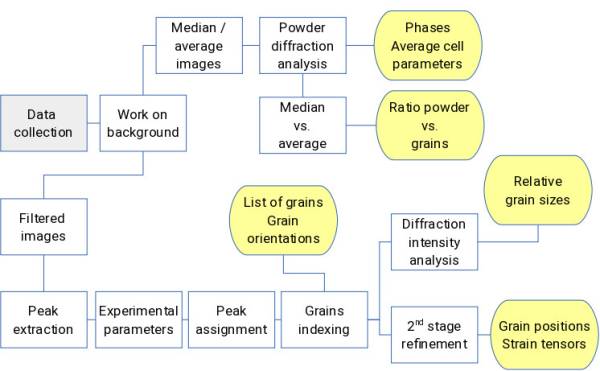
Here is an outline of a data processing workflow. This assumes that you already have your data collected. Depending on your objectives, follow the matching track.

The scripts and software you should use for each step are

• Data: you should look at your diffraction data with Fabian. Pay attention about image orientation and rotation. You can also start looking at diffraction intensity levels, in the background, in the peaks, etc.
• Generating backgrounds, median, average images: Image Math.
• Looking at images with background subtracted: Fabian.
• Peak extraction: Peaksearch
• To be completed…

1. Create an input file with the ending .inp. It should contain information on instrumentals of the experiment, the grain, the sample, strain, background, peak shape, and so on. You find an example of an input file here.
2. Next you can run the simulation with PolyXSim. This simulation may take a while…
3. Afterwards, you can look at the output with Fabian.
4. If you have “real” data, this would be the point when you work on the background (more information on this topic here). If you also simulated noise, strain or other things that make your data look more like “real” data, it might be useful to do a background substraction, too.
5. Now you can search for peaks using the software PeakSearch.
6. In ImageD11 the found peaks are fitted to the parameters of the sample and experiment, followed by the calculation of the g-vector.
7. With the calculated g-vector, the grains will now be indexed, using GrainSpotter.
8. The calculated grains should then be compared and checked with the simulated grains.

The purpose of this step is to simulate the outcome of a DAC experiment (grains with random orientations, random strains etc.). It is a possibility to check outcome of an actual experiment. The simulation will not only provide 2D diffraction images but also G-vectors, inverse Ub matrices and some more files. You will get at least 7 different files from the simulation plus the diffraction images. The amount of diffraction images depends on the ω range and the step size you put into the input file. For example, a ω range from -28° to +28° with a step size of 0.5° produces 112 images (numbers from 0 to 111).

Create an input file with the ending .inp. For a start, simply modify an existing one like this. Afterwards, you can run the simulation with PolyXSim. Write the following to the Konsole:

PolyXSim.py -i 'some_input_file'.inp

The 7 different files (which were just mentioned above) are usually created quite fast. The time consuming process is the creation of images. This time highly depends on the parameters you put in the input file, e.g. the amount of grains, the peak shape and if you switched on strain tensors or noise. If you just want to test if the software is working it is wise to use an input file with very simple parameters (only 1 grain, no strain tensors, no noise, small ω range etc.).

While the simulation is running you can already look at the images, which are already created. For this, open a new tab in the Konsole and open Fabian:

fabian.py

This is convenient because you can already see at this point if your simulation works. And in case it does not, you can stop the simulation process right now and you don't need to wait until all images are created, which can take very long time. While you're at it, check also the O-matrix. You find it in Fabian under Image –> Orientation. Choose the one which is the same as in your input file.

To get rid of the background we now add up all the diffraction images and calculate an average and a median image. Then, every image is subtracted by this average/median image which should remove the background. Of course, if you switched off the background in the previous simulation this process won't change anything. But in case you have real data, this procedure is essential!

For calculating the average and median you use Image Math. Type to the Konsole:

image_math_petra 'name stem of the .edf file' 'first image number' 'last image number' median
or
./image_math_petra.bin 'name stem of the .edf files including their directory path' 'first image number' 'last image number' median

For more information on which syntax you should use, check the Image Math wiki page. The calculation will create three additional .edf files which are automatically stored in the same folder. They share the same name with the other .edf files except for an additional letter m (for median) in the middle of the name. So look carefully not to oversee them. The images are numbered from 1 to 3.

• Image m1 is the average image
• Image m2 is the median image
• Image m3 is the ?? image

Since they are also .edf images, you can also have a look at them with Fabian if you like. Next, the actual images have to be subtracted by one of these three images. Usually the m2 image (median) is used for this, because it is less affected by outliers. Before you do this, make sure you have a separate folder to avoid mixing up the actual data with the processed data! Raw data should never be modified!

Look at the images in Fabian, go to Image –> Correction –> Subtract background and choose the m2 image. Now every image which is currently loaded (including those which you can access by clicking on next and previous) gets subtracted by this m2 image (median). If it is not simulated data without noise etc. you should see a difference. The peaks should appear clearer.

From these processed images you can now extract the peaks. Look at some random peaks from several images by zooming in (in Fabian) and check out their intensity. Try to estimate a threshold value which defines how intense a peak must be to be seen by the algorithm. Try to define a threshold, which separates peaks from background (everything above the threshold value is a peak, everything below is background). If you are not sure you can also define several threshold values.

When you defined one (or more) threshold(s) you can start the PeakSearch algorithm:

peaksearch.py -n ../'directory'/'name stem' -f 'number of first image' -l 'number of last image' ../'directory'/'median .edf file' -t 'threshold value 1' -t 'threshold value 2' ...

To check the outcome of PeakSearch, you can load the peaks, which were found, into Fabian and see if they match the actual peak positions.