Table of Contents
Plotting grain orientations
Typically, grain orientations are plotted with MTeX based on the Euler angles of each grain.
Extracting Euler angles
Extracting a list of Euler angles for the indexed grains can be done using timelessExtractEulerAngles, which is part of the TIMEleSS tools.
You will have a list of Bunge Euler angles (using a Bunge convention) as below. You can simply save it in a text file.
-31.88 273.49 206.05
-55.09 133.91 157.65
83.39 235.30 204.46
-47.58 78.99 149.71
-60.87 17.28 33.07
Loading and plotting grain orientations in MTeX
Here is an example of a script that will load these orientations and plot them in a pole figures. The example is for olivine and can be adjusted to your needs.
- plotGrainPF.m
%%
% Define crystal and sample symmetry
cs_ol = crystalSymmetry('Pnma',[9.915267 5.886196 4.713400])
ss = specimenSymmetry()
% Plotting convention
plotx2east
% File with Euler angles
fname = fullfile('/path/to/folder/',...
    '','euler.txt');

%%
% Load file and create the corresponding list of orientations
ori = load(fname)
n = size(ori);
n = n(1);

for i = 1:n
    phi1 = ori(i,1)*degree;
    Phi = ori(i,2)*degree;
    phi2 = ori(i,3)*degree;
    ori0(i) = orientation('Euler',phi1,Phi,phi2,cs_ol,ss);
end

%%
% Plot grain orientations
h = Miller({1,0,0},{0,1,0},{0,0,1},cs_ol)
plotPDF(ori0,h,'antipodal','MarkerSize',10, 'MarkerFaceColor', 'b', 'MarkerEdgeColor', 'b')
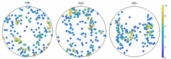
Loading and plotting grain orientations in MTeX, with colors!
Here is an example of a script that will load these orientations and plot them in a pole figures. The example is for olivine and can be adjusted to your needs.
In this case grains are assigned a color based on the ODF intensity for their orientations.
- plotColorGrainPF.m
%%
% Define crystal and sample symmetry
cs_ol = crystalSymmetry('Pnma',[9.915267 5.886196 4.713400])
ss = specimenSymmetry()
% Plotting convention
plotx2east
% File with Euler angles
fname = fullfile('/path/to/folder/',...
    '','euler.txt');

%%
% Load file and create the corresponding list of orientations
ori = load(fname)
n = size(ori);
n = n(1);

for i = 1:n
    phi1 = ori(i,1)*degree;
    Phi = ori(i,2)*degree;
    phi2 = ori(i,3)*degree;
    ori0(i) = orientation('Euler',phi1,Phi,phi2,cs_ol,ss);
end

%%
% Plots grains using a color scale base on ODF fitted to the grains

% Fit an ODF to the data
odf = calcODF(ori0,15*degree)

% Plot orientations, colored based on ODF
plotPDF(ori0,eval(odf,ori0),h,'antipodal','MarkerSize',10, 'MarkerEdgeColor', 'b')
CLim(gcm,[0,10])
mtexColorbar
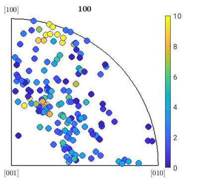
Loading and plotting grain orientations in MTeX, in an inverse pole figure, and with colors!
Here is an example of a script that will load these orientations and plot them in a inverse pole figures. The example is for olivine and can be adjusted to your needs. Grains are assigned a color based on the ODF intensity for their orientations.
- plotColorGrainIPF.m
%%
% Define crystal and sample symmetry
cs_ol = crystalSymmetry('Pnma',[9.915267 5.886196 4.713400])
ss = specimenSymmetry()
% Plotting convention
plotx2east
% File with Euler angles
fname = fullfile('/path/to/folder/',...
    '','euler.txt');

%%
% Load file and create the corresponding list of orientations
ori = load(fname)
n = size(ori);
n = n(1);

for i = 1:n
    phi1 = ori(i,1)*degree;
    Phi = ori(i,2)*degree;
    phi2 = ori(i,3)*degree;
    ori0(i) = orientation('Euler',phi1,Phi,phi2,cs_ol,ss);
end

%%
% Plots grains using a color scale base on ODF fitted to the grains

% Fit an ODF to the data
odf = calcODF(ori0,15*degree)


% Plot grains as IPF of the compression (if compression is in X), colored based on ODF
plotIPDF(ori0,eval(odf,ori0),[vector3d.X],'antipodal','MarkerSize',10, 'MarkerEdgeColor', 'b')
CLim(gcm,[0,10])
mtexColorbar
Comparing grain orientations in MTeX
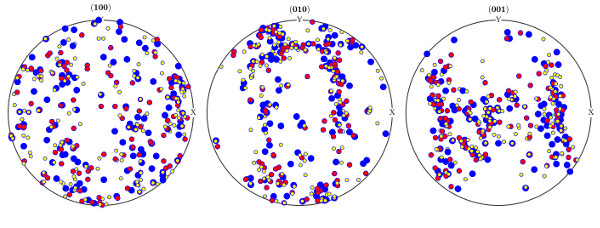
The following script will load results from 3 different indexings a plot the results so they can be compared.
The image below for instance shows the results of a first indexing in blue, a second indexing in red, and a third indexing in yellow.
- compareGrainPF.m
%%
% Define crystal and sample symmetry
cs_ol = crystalSymmetry('Pnma',[9.915267 5.886196 4.713400])
ss = specimenSymmetry()
% Plotting convention
plotx2east
% Files with Euler angles
fname1 = fullfile('/path/to/folder/',...
    '','euler-1.txt');
fname0 = fullfile('/path/to/folder/',...
    '','euler-2.txt');
fname2 = fullfile('/path/to/folder/',...
    '','euler-3.txt');

%%
% Load file and create the corresponding 3 lists of orientations
ori = load(fname0)
n = size(ori);
n = n(1);

for i = 1:n
    phi1 = ori(i,1)*degree;
    Phi = ori(i,2)*degree;
    phi2 = ori(i,3)*degree;
    ori0(i) = orientation('Euler',phi1,Phi,phi2,cs_ol,ss);
end

ori = load(fname1)
n = size(ori);
n = n(1);

for i = 1:n
    phi1 = ori(i,1)*degree;
    Phi = ori(i,2)*degree;
    phi2 = ori(i,3)*degree;
    ori1(i) = orientation('Euler',phi1,Phi,phi2,cs_ol,ss);
end

ori = load(fname2)
n = size(ori);
n = n(1);

for i = 1:n
    phi1 = ori(i,1)*degree;
    Phi = ori(i,2)*degree;
    phi2 = ori(i,3)*degree;
    ori2(i) = orientation('Euler',phi1,Phi,phi2,cs_ol,ss);
end

%%
% Plot grain orientations from the 3 files in a way they can be compared
h = Miller({1,0,0},{0,1,0},{0,0,1},cs_ol)
plotPDF(ori0,h,'antipodal','MarkerSize',10, 'MarkerFaceColor', 'b', 'MarkerEdgeColor', 'b')
hold on
plotPDF(ori1,h,'antipodal','MarkerSize',8, 'MarkerFaceColor', 'r', 'MarkerEdgeColor', 'b')
hold on
plotPDF(ori2,h,'antipodal','MarkerSize',6, 'MarkerFaceColor', 'y', 'MarkerEdgeColor', 'b')


